Tutorial

This tutorial shows how to use LIRICAL to evaluate an exome.

Setup

Follow the instructions in Setting up LIRICAL to install the Exomiser database. Note the location of the Exomiser database (it will be needed to run LIRICAL, see below). Most users should download the pre-built version of LIRICAL available on the Releases page. Instructions are also offered for building LIRICAL from source if desired.

The data

We have simulated an exome VCF file by adding a disease associated variant to a VCF file derived from project.NIST.hc.snps.indels.NIST7035.vcf. A disease-associated mutation in the TGFBR2 gene (see Patient 4 in Cao et al., 2018) was spiked into the VCF file.

Download the VCF file (LDS2.vcf) from Figshare.

Creating a phenopacket

Here is an excerpt of the text that described patient 4 in the above cited article:

Patient  4  is  a  9-year-old  girl.  She  was  clinically  diagnosed  with  suspected
Marfan syndrome  according  to  the  first  impression.  She  was  144  cm  tall and
weighed  24  kg.  Her  father  was  176  cm  tall  and  weighed 53  kg.  The  phenotypes
of  this  patient  include strabismus, refractive  error, pectus  carinatum,  scoliosis,
arachnodactyly, and camptodactyly. The patient's main cardiovascular abnormalities
were Sinus of Valsalva aneurysm, aortic root dilation, aortic regurgitation,
atrial septal defect, patent foramen ovale, pulmonary artery dilatation, and
tricuspid valve prolapse with regurgitation. Craniofacial abnormalities of the
patient include bifid uvula, malar hypoplasia, and micrognathia.

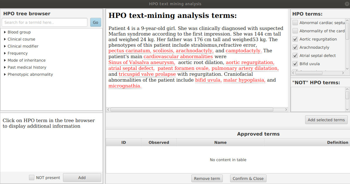
Use the PhenopacketGenerator to create a Phenopacket.

To set up PhenopacketGenerator, you will first need to set the location of the hp.obo file. Download hpo.obo from the Download page of the HPO website. Enter your Biocurator id by selecting “Set biocurator id” from the edit menu, and enter an arbitrary Phenopacket ID and proband ID. Use the dropdown menus to enter “9 years” for Age and “Female” for sex.

From the edit menu, select “Set path to hp.obo file”, then select the location of the hpo.obo on your computer. After a moment, the ontology will load and “Enter HPO terms” will be clickable. Load HPO terms for this case by clicking “Enter HPO term”. Paste the clinical description above into the text-mining window of PhenopacketGenerator, click “Analyze”, select HPO terms, click “Add selected terms”, then “Confirm and Close”.

Then, select the location of the VCF file that you saved in the previous step, and enter the Genome assembly (hg19).

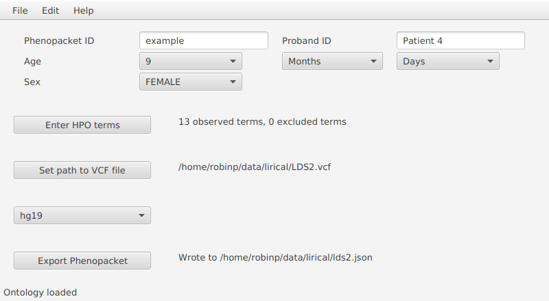
You can now export the phenopacket. Use the filename LDS2.json (or choose another name and adjust the following command accordingly).

Running LIRICAL

Run LIRICAL as follows.

$ java -jar LIRICAL.jar phenopacket -p LDS2.json  -e /path/to/exomiser-data/ -x LDS2

Viewing the results

The above command will create a new file called LDS2.html (the -x option controls the prefix of the output file). Open this file in a web browser. The top of the page shows some information about the input files and a list of observed and excluded HPO terms. The next section shows summarized representations of the top candidates.

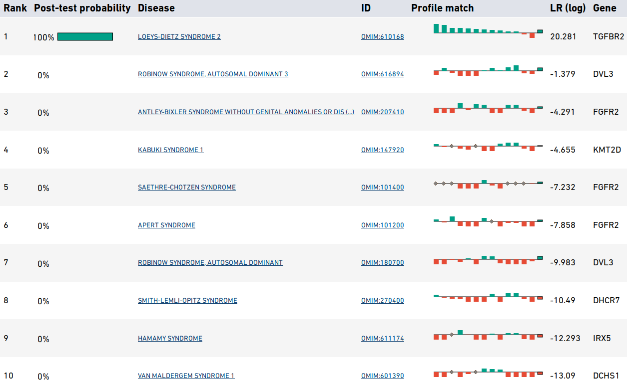
Summary view of the top candidates.

Each row in the summary shows the rank, post-test probability, and name/ID of the disease. The row includes a sparkline representation of the phenotypic profiles of each candidate, with green bars indicating positive contributions and red bars negative contributions to the diagnosis. The last bar represents the genotype likelihood ratio if LIRICAL was run with a VCF file. Mousing over the individual bars will show the name of the HPO term or gene, and all sparklines show the terms in the same order.

LIRICAL then presents a detailed analysis of each of the top candidates. The summary shows information about identified variants and the phenotypic profile. Mousing over the graphic shows information about the likelihood ratio and the type of the match.

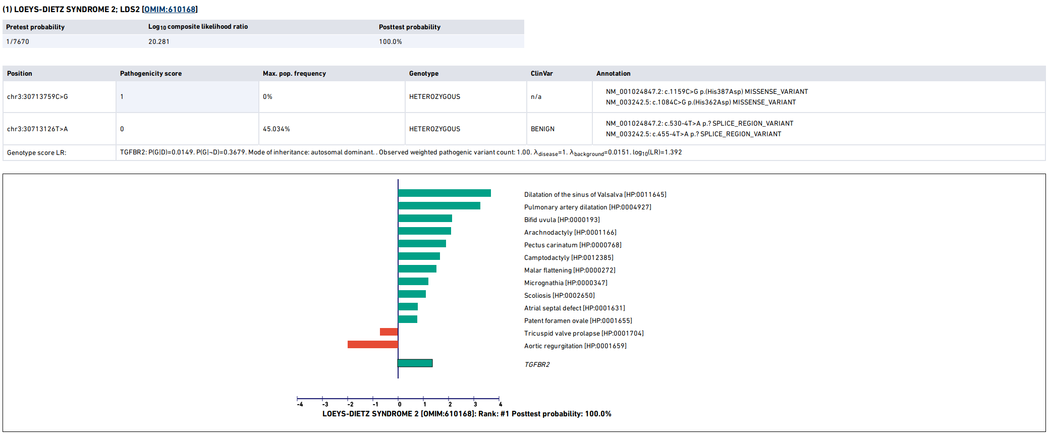
Detailed view of the top candidate Loeys-Dietz syndrome type 2.

The remaining part of the HTML output page contains information about the other top candidates and a list of all diseases analyzed. The bottom of the page includes explanations and documents the settings used for the analysis.